Pipelining in Computer Architecture

Pipelining

Let’s recall the processor design. The first simple processor design is executed in one clock cycle. It is also known as a single-cycle processor. However, the single-cycle processor is not practical in real implementation since the memory operations cannot execute in one clock cycle as well as the arithmetic operations have high propagation delay. Consequently, the multi-cycle processor is invented, in which it divides the single-cycle processor into many stages. The maximum clock frequency that it can operate depends on the longest path or longest stage, which is absolutely smaller than a single-cycle processor.

Computer architects are always wondering how to build faster computers. To define how fast the computer is, the cycle per instruction (CPI) is introduced. The cycle means the one clock frequency, which depends on the critical path for each processor. In general, to compare two or more processors, the time/program is compared. The time/program is defined as:

\[\frac{time}{program} = \frac{\#instructions}{program} \times \frac{cycles}{instruction} \times \frac{time}{cycle}\]

The instructions per program depend on source code, compiler technology, and the instruction set architecture (ISA). The CPI depends on the microarchitecture design. All we want is to get all the terms as small as possible. We actually cannot change the value of instructions per program. Thus, a computer architect needs to optimize CPI and clock frequency. For example, a single-cycle processor can have a CPI equal to one, but the cycle time is high. Meanwhile, a multi-cycle can have a low cycle time, but the CPI is more than one. A pipeline processor is introduced and claims that it has a CPI equal to one and the clock period is low.

Pipeline Processor

Pipeline processor takes the multicycle processor stage into a pipeline manner which means the stage is execute and finish in sequence. Similar to the pipeline model, the second instruction does not need to wait until the first instruction finish. It needs to wait for the first instruction finish the first stage which probably one clock cycle. Based on this scenario, if the pipeline is full, the CPI of pipeline processor would equal to one and the clock cycle is similar to multicycle processor which is low. Therefore, pipeline processor would potentially fast than nonpipelined.

The multicycle processor divides the processor typically in 5 stages:

Instruction Fetch
Instruction Decode
Execute
Memory
Writeback

drawing

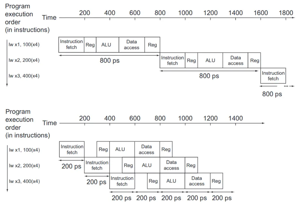
The figure shows the difference between multicycle process execution and pipeline process execution. It shows that the non-pipelined processor takes 800 ps to execute one instruction, while executing one instruction in a pipeline processor takes 1000 ps. However, a pipeline processor can execute multiple instructions in parallel, which consequently reduces the overall program execution time. It can clearly be seen that the pipeline processor takes 1400 ps while the non-pipeline takes 2400 ps to execute three instructions.

Pipeline Hazards

There are some situations in which the instruction cannot continue in the pipeline processor. We call this hazards, and there are three types of hazards: structural hazard, data hazard, and control hazard.

The structural hazard means that the hardware architecture cannot perform the next instructions, and it needs to wait until the prior instruction is finished. Normally, this is not occur in RISC machine since it desing to be pipelinable. However, it can be limited by the number of memory ports. For example, if the memory port is one, which means the instruction fetch and memory stage cannot execute at the same time, the instruction needs to wait until it has been fetched or the memory is read or written. Basically, provided that we utilized dual port memory, it would not be a problem.

The data hazards occur when the next instruction uses the same register as the current instruction. We call this data dependencies. For example, we have lw x1, x8, and addi x9, x1, 20. The load word instruction loads some value to the x1 register, while the next instruction wants to add value in x1 with 10. If these two instructions execute independently, the value we get in x9 would be incorrect since x1 is not the value in memory. Conventionally, we need to wait until the first instruction is finished. Nonetheless, we can do better with the data forwarding technique, which said that it will bypass the data from where it is done back to where it needs to be. In this case, x1 is done in the memory stage, and it would be a straightforward bypass to execute the stage for the addi instruction. Thus, the processor needs to stall or wait for only one cycle instead of 3 cycles.

Last but not least, control hazards occur when we make a decision, normally a branch. Imagine that we execute instructions in a pipeline manner, and the branch decision is desired in the execute stage. It may result in the executed instructions being incorrect since the branch desires to branch or jump to some instruction address that is not the current instruction address. To solve this, the pipeline should be able to flush the instruction if it executes the wrong instruction, or the pipeline would stall if the branch instruction is executed. To reduce the stall time, the branch prediction would be applied.

Conclusion

We show that the pipeline is invented to reduce the CPI and maintain a low clock period. However, there are some hazards that tend to increase the CPI. The data hazards are solved efficiently by data forwarding. The control hazard simply stalls or flushes the instruction until it determines to take or not take a branch. The branch prediction would be used to reduce the CPI as well.

Reference

David A. Patterson, John L. Hennessy. 2021. Computer Organization and Design RISC-V Edition The Hardware Software Interface. The Morgan Kaufmann Series in Computer Architecture and Design.